State Analysis

Lower output does not automatically mean that a machine is operating too slowly. Time is often lost due to waiting, setup, or recurring interruptions. The state analysis shows how the available time is distributed among these operating states and when the losses occur.

You can see both the percentages over a period of time and the trends for individual stages. This allows you to determine whether production is being affected by a single long disruption or many short interruptions.

Classify Machine States in an Easy-to-Understand Way

Control systems use different status codes. What is referred to as “Automatic” on one machine may be described by multiple signals on another. To enable consistent evaluation, these raw statuses are mapped to technically meaningful statuses during configuration.

Typical groups include Production, Maintenance, Setup, and Malfunction. You determine which groups are appropriate for your plant and which raw statuses belong to them. The status hierarchy and aggregations determine how this information is consolidated for evaluation.

This classification creates a common foundation for production and maintenance. As a result, a long wait time is not mistakenly interpreted as a technical defect. Different machines can be viewed at the same technical level.

Compare Time Allocations

The status distribution shows the duration and proportion of each status during the selected time period. It provides a useful initial overview: Was the plant primarily in production? Was a significant amount of time spent on setup? What percentage of the time was spent on malfunctions or downtime?

Start with the largest relevant time component. For example, if waiting time accounts for the majority of the loss, examining the material supply or adjacent workstations may be more helpful than looking for shorter processing cycles.

Be sure to consider the actual number of minutes. A similar percentage can result in a significantly larger loss when the production period under consideration is longer.

Understanding Interruptions Over Time

The timeline and heat map show when conditions occur and how they follow one another. While the distribution shows the extent, the progression explains the structure of the loss.

Visible in the course of the process	Approach to the study
A long service disruption	Investigate the specific incident and related reports.
Frequent short cycles between production and disruptions	Check for recurring interruptions and their causes.
Longer wait times	Consider material flow and upstream or downstream stations.
Recurring setup phases	Align the process with the planned product changes.

Two facilities may have the same downtime rate but still require very different measures. The trend helps identify this difference early on.

Recognizing Patterns in the Line

The line overview summarizes the statuses of the associated plants. By comparing the time series of adjacent stations, it is possible to determine where an outage begins and which stations subsequently stop producing as well.

This is particularly helpful in waiting states. A station in a waiting state does not necessarily have to have an error itself. It may be missing material because an upstream station has been interrupted. Similarly, a downstream process may block the transfer.

Therefore, evaluate station and line times separately. If three stations come to a standstill for ten minutes at the same time, the line does not automatically lose thirty minutes as a result. The timing relationships are crucial.

Example: A malfunction at one station is followed by delayed wait times at other stations. The overall sequence provides a starting point for investigating the cause. Open full-size graphic (new tab)

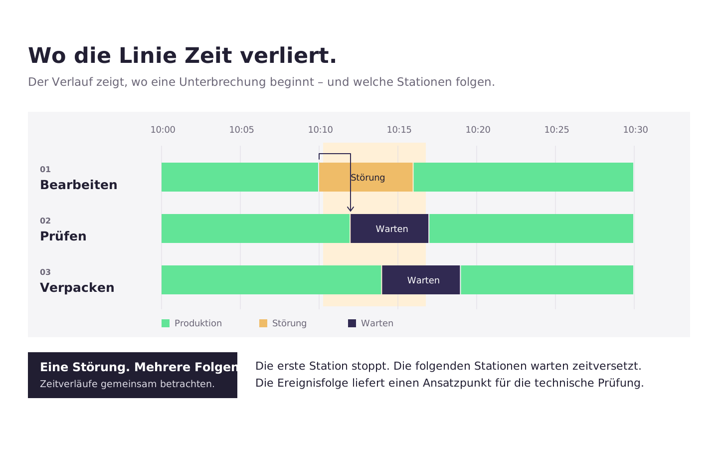
Examine a time period with reports

For a segment that stands out, you can view the associated messages, provided that the corresponding event and alarm log is assigned to it. The event analysis supplements the status history with errors, warnings, and other events.

This is how the request to the maintenance department can be specified: instead of “The station is often down,” for example, “These recurring interruptions all begin during a period marked by the same sequence of error messages.” The technical cause is then investigated based on these events.

Example: The waiting station is not the starting point

A station has a high proportion of waiting time. At first glance, it seems likely that there is a problem there.

1. Check the scope. Examine the duration and percentage of time spent in the waiting state during the selected time period.
2. View wait times. Check the history to see whether the time is accumulated in one long period or many short periods.
3. Compare neighboring stations. Examine what happens at the upstream station shortly before these phases begin.
4. Investigate the notable incident. If a fault has occurred repeatedly prior to this, review the corresponding messages for these sections.
5. Monitor the effect. After implementing a measure at the upstream station, check whether the wait time at the following station has also decreased.

This helps to begin the analysis at the point where the interruption occurred, rather than solely at the station with the most significant portion of the time.

Data Set and Time Evaluation

The analysis uses the assigned machine state log. Check the setup against a known production run and a known downtime period. Do the status, start time, and duration match the actual sequence of events?

To begin an evaluation period, it must be known which state was already active. Furthermore, missing state data or connection interruptions do not constitute evidence of downtime. They must remain identifiable as unknown time so that the evaluation does not confuse data collection with plant behavior.

The state analysis also provides a basis for the availability factor in the OEE calculation. There, it is also determined which periods are considered part of the planned production time and how the individual states are evaluated.